Personal City-Level Location Prediction Based on Behavior via Machine Learning
, Munich
Before I started my Erasmus I thought it could be fun to collect some data about myself while traveling so that I can visualize and analyze them later.
Here I will try to do exactly that without diving into any theoretical explanations of why I did what I did, but I'll add some interpretations of the results.
Goals
This post has two goals:
- Explore and visualize my personal data from my Erasmus time (and a bit after)
- Predict the city I am in based on my behavior (number of steps on a day, money spent, and number of photos/videos taken)
For goal 1, I will use data I collected myself from my phone and smartwatch, as well as data that Google collected about me.
For goal 2, I will use only the data that I collected myself.
I'll consider goal 2 a success if I can feed in the following day that wasn't part of the training data and get a prediction that is correct.
On December 19, 2023 I was in Munich, I took 2575 steps, spent no money, and took no photos/videos.
example = {
    'steps': 2575,
    'money_spent_offline': 0,
    'money_spent_online': 0,
    'money_spent_total': 0,
    'photos_videos': 0
}
I don't aim to get the best results possible, but rather to get a rough idea of how well this can work and I don't aim to explain any theory.
Exploration and Visualization
Google Data
Let's start by exploring some of the data that Google saved about me. In total, Google saved 2164 place visits.
All map data used for images © OpenStreetMap contributors
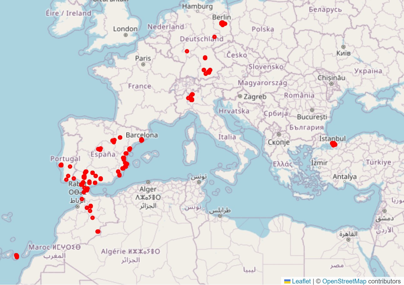
These are the top 5 places I visited repeatedly and the number of times I have been there:
El Viajero Sedentario         163
University of Seville          66
Torneo (San Lorenzo)           31
Quiero Dulce                   21
REWE                           20

...                          ...

Giselastraße                    1
German post office              1
Gazzo                           1
Garching-Forschungszentrum      1
La Sagrada Familia              1
Google only saves the names of visited places, but doesn't categorize them. I tried categorizing by place name and what the name contains. This is very inaccurate, as lots of places won't have their category in their name. E.g., cafés often won't have "café" in their name.
What should be accurate is at least my home addresses, university, and airport visits. The airport visits don't all correspond to flights, but also include picking up or dropping off friends.
Here's the result:
Other            1258
Seville Home      483
Munich Home        74
University         73
Market             51
Cafe               42
Airport            40
Berlin Home        38
Train Station      33
Bar                32
Restaurant         23
Beach               9
Museum              8
Google can also save activities it recognizes like flying, walking, bus rides, etc.
This is what the first five entries of the activity data set look like (some coordinates censored):
      activityType
      startTimestamp
      endTimestamp
      startLatitude
      startLongitude
      endLatitude
      endLongitude


      473
      IN_PASSENGER_VEHICLE
      2022-09-01 02:20:28.243000+00:00
      2022-09-01 03:04:01+00:00
      ?????
      ?????
      52.365605
      13.508949


      474
      FLYING
      2022-09-01 04:23:15.995000+00:00
      2022-09-01 06:10:42.876000+00:00
      52.365978
      13.505437
      50.044165
      8.562142


      475
      FLYING
      2022-09-01 07:18:53.480000+00:00
      2022-09-01 10:23:56.245000+00:00
      50.044132
      8.562804
      37.423092
      -5.899401


      476
      IN_PASSENGER_VEHICLE
      2022-09-01 10:57:11.553000+00:00
      2022-09-01 11:16:23.291000+00:00
      37.423862
      -5.900755
      37.381626
      -6.000961


      477
      WALKING
      2022-09-01 11:37:37.062000+00:00
      2022-09-01 12:08:41.935000+00:00
      37.382230
      -6.001706
      ?????
      ?????
So now it is possible to plot the activities on a map.
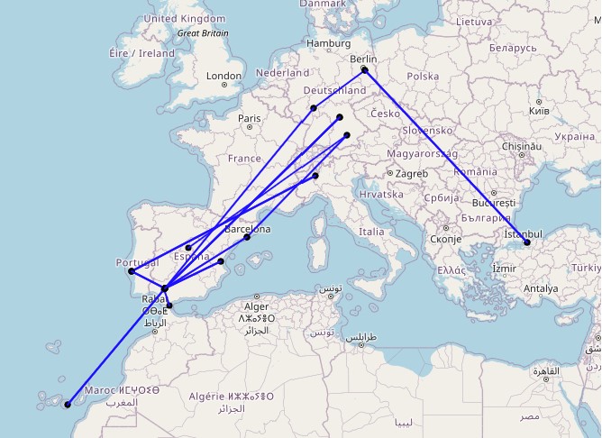
Flights
Here are all my flight connections:
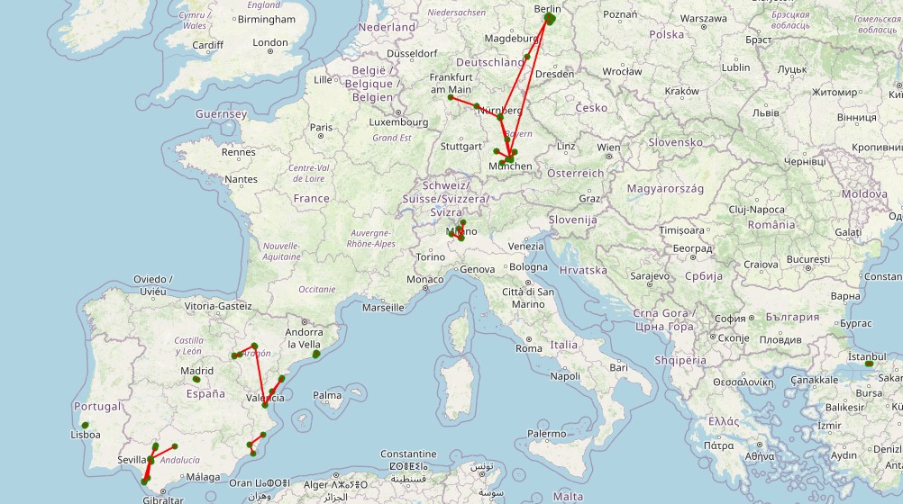
Train Rides
All train rides:
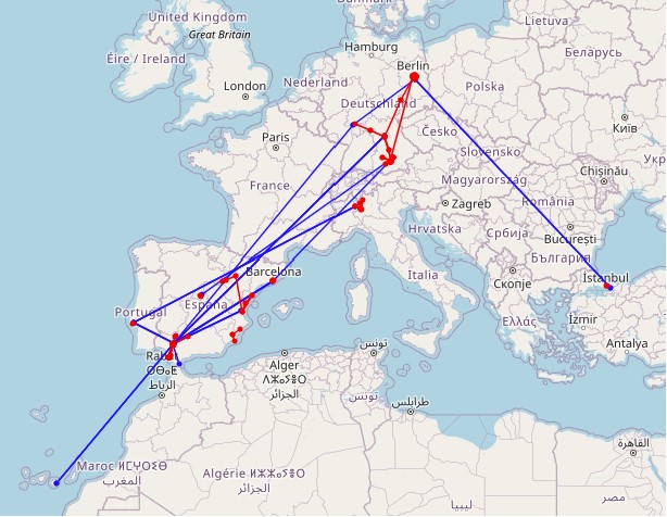
Flights and Train Rides
Flights and train rides combined:
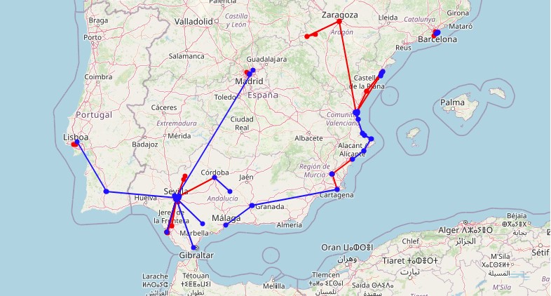
Bus and Train Rides
A few of the bus rides were mixed up with train rides, so I'll show train rides and bus rides combined:
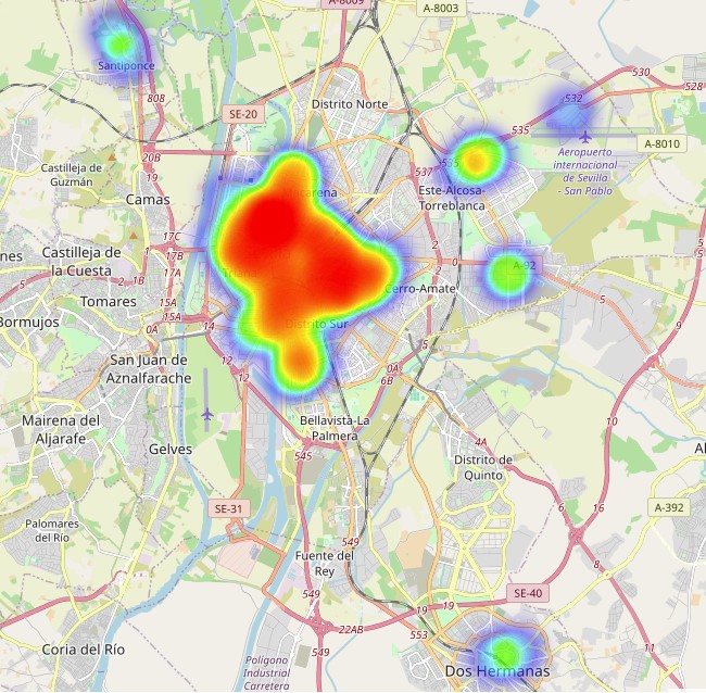
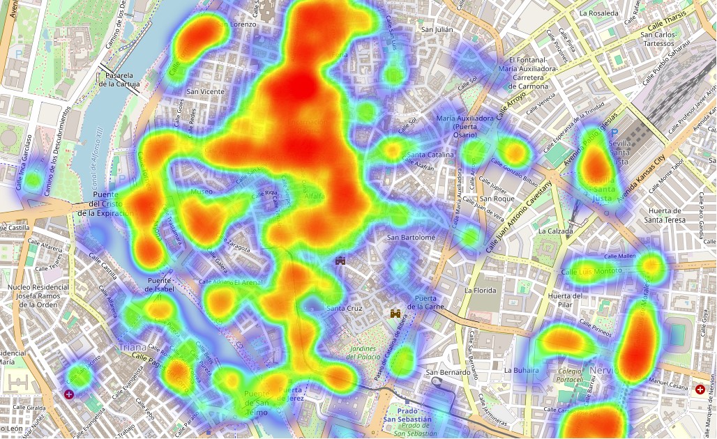
Walking
For walking, here are heatmaps of where I walked most in Sevilla, first zoomed out and then closer:
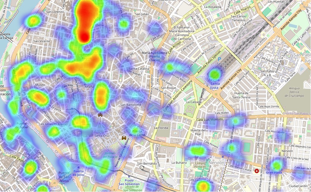
For the place visits Google saves, it looks rather similar to the walking heatmap, as I mostly walked everywhere anyway:
My own data
Originally, the data I collected about myself contained rows for about every half hour. It recorded my coordinates, the location name on a city level, the country name, the number of Wi-Fi networks in reach, and a timestamp.
I aggregated this to one row per day for simplicity. Then I needed to assign a single city to each day, which leads to some places where I spent little time to not show up in the data.
Then I added more columns: I scraped my bank account for my payments history, processed my smartwatch data for heart rate, counted my photos and videos, and used a weather service for temperature and condition data.
As my phone broke and I didn't have one for a few days, I also filled in some missing data manually or, as in the case of steps for example, filled in the mean of the variable. This might introduce bias, but as there were only a few days missing, I think it's acceptable.
In the end I also added some augmented data, e.g., the day of the week, season, or a simplified weather condition.
This is, in short, how I arrived at the dataset I will use.
The final dataset contains 416 rows and 30 columns. I think the most interesting columns here are
date, city, max_temp, apparent_max_temp, weather_condition, steps, money_spent_offline, money_spent_online, wifi_count_mean, heart_rate_combined, photos_videos
All temperature values are in °C, money spent in €, and heart rate in bpm.
These are the first 10 rows (days) of the dataset:
      weekday
      weekend
      month
      season
      city
      country
      max_temp
      apparent_max_temp
      temp_difference
      humidity
      weather_condition
      simplified_weather
      steps
      activity
      money_spent_offline
      money_spent_online
      money_spent_total
      wifi_count_mean
      watch_1_steps
      watch_2_steps
      watch_steps_combined
      watch_1_mean_heart_rate
      watch_2_mean_heart_rate
      heart_rate_combined
      watch_type
      photos_videos
      media_activity
      generic_lat
      generic_lon


      date


      2022-08-25
      Thursday
      Weekday
      August
      Summer
      Berlin
      Germany
      27.3
      28.7
      -1.4
      Moderate
      Light drizzle
      Rain
      10399
      Moderate
      7.20
      0.00
      7.20
      9.25
      NaN
      NaN
      NaN
      NaN
      NaN
      NaN
      NaN
      0
      NaN
      52.52437
      13.41053


      2022-08-26
      Friday
      Weekday
      August
      Summer
      Berlin
      Germany
      26.9
      29.2
      -2.3
      Humid
      Heavy rain
      Rain
      3991
      Low
      0.00
      0.00
      0.00
      11.57
      NaN
      NaN
      NaN
      NaN
      NaN
      NaN
      NaN
      1
      Moderate
      52.52437
      13.41053


      2022-08-27
      Saturday
      Weekend
      August
      Summer
      Berlin
      Germany
      23.0
      25.1
      -2.1
      Humid
      Moderate rain
      Rain
      2423
      Low
      0.00
      0.00
      0.00
      2.79
      NaN
      NaN
      NaN
      NaN
      NaN
      NaN
      NaN
      1
      Moderate
      52.52437
      13.41053


      2022-08-28
      Sunday
      Weekend
      August
      Summer
      Berlin
      Germany
      21.9
      20.8
      1.1
      Moderate
      Light drizzle
      Rain
      2143
      Low
      0.00
      0.00
      0.00
      9.46
      NaN
      NaN
      NaN
      NaN
      NaN
      NaN
      NaN
      5
      Moderate
      52.52437
      13.41053


      2022-08-29
      Monday
      Weekday
      August
      Summer
      Berlin
      Germany
      21.7
      20.9
      0.8
      Moderate
      Light drizzle
      Rain
      8250
      Moderate
      9.95
      0.00
      9.95
      12.47
      NaN
      NaN
      NaN
      NaN
      NaN
      NaN
      NaN
      9
      Moderate
      52.52437
      13.41053


      2022-08-30
      Tuesday
      Weekday
      August
      Summer
      Berlin
      Germany
      20.9
      20.4
      0.5
      Moderate
      Light drizzle
      Rain
      6856
      Moderate
      15.95
      0.00
      15.95
      7.83
      NaN
      NaN
      NaN
      NaN
      NaN
      NaN
      NaN
      0
      NaN
      52.52437
      13.41053


      2022-08-31
      Wednesday
      Weekday
      August
      Summer
      Berlin
      Germany
      21.3
      19.7
      1.6
      Moderate
      Light drizzle
      Rain
      10668
      Moderate
      0.00
      0.00
      0.00
      21.10
      NaN
      NaN
      NaN
      NaN
      NaN
      NaN
      NaN
      0
      NaN
      52.52437
      13.41053


      2022-09-01
      Thursday
      Weekday
      September
      Autumn
      Seville
      Spain
      34.7
      33.4
      1.3
      Moderate
      Mostly cloudy
      Cloudy
      28784
      High
      76.96
      0.00
      76.96
      21.83
      NaN
      NaN
      NaN
      NaN
      NaN
      NaN
      NaN
      30
      High
      37.38283
      -5.97317


      2022-09-02
      Friday
      Weekday
      September
      Autumn
      Seville
      Spain
      33.6
      31.9
      1.7
      Moderate
      Partly cloudy
      Cloudy
      13744
      High
      34.28
      21.00
      55.28
      15.05
      NaN
      NaN
      NaN
      NaN
      NaN
      NaN
      NaN
      14
      Moderate
      37.38283
      -5.97317


      2022-09-03
      Saturday
      Weekend
      September
      Autumn
      Seville
      Spain
      32.1
      31.0
      1.1
      Moderate
      Mainly clear
      Clear
      35051
      High
      42.00
      71.93
      113.93
      12.60
      NaN
      NaN
      NaN
      NaN
      NaN
      NaN
      NaN
      58
      High
      37.38283
      -5.97317
I visited at least the following 28 cities. The count is the number of days I spent there.
There are cities missing, like Ronda for example, because I didn't spend a lot of time there. I didn't bother to fix this.
Seville                       223
Munich                         65
Berlin                         48
Cádiz                          21
Istanbul                        7
Milano                          6
Lisbon                          4
Madrid                          4
Valencia                        4
Barcelona                       4
Las Palmas de Gran Canaria      3
Vinaròs                         3
Merzouga                        3
Benidorm                        3
Cartagena                       2
Córdoba                         2
Alhama de Aragón                2
Fès                             2
Dénia                           1
Zaragoza                        1
Castelló de la Plana            1
Lagoa                           1
Granada                         1
Málaga                          1
Zuheros                         1
Barbate                         1
Jerez de la Frontera            1
Santiponce                      1
And these are the 6 countries I visited (on 3 continents, two of which I visited for the first time):
Spain       280
Germany     113
Turkey        7
Italy         6
Portugal      5
Morocco       5
The following are some summary statistics like top value per variable, mean, or min and max. I censored the money_spent variables as I will also do later on.
      weekday
      weekend
      month
      season
      city
      country
      max_temp
      apparent_max_temp
      temp_difference
      humidity
      weather_condition
      simplified_weather
      steps
      activity
      money_spent_offline
      money_spent_online
      money_spent_total
      wifi_count_mean
      watch_1_steps
      watch_2_steps
      watch_steps_combined
      watch_1_mean_heart_rate
      watch_2_mean_heart_rate
      heart_rate_combined
      watch_type
      photos_videos
      media_activity
      generic_lat
      generic_lon


      count
      416
      416
      416
      416
      416
      416
      416.000000
      416.000000
      416.000000
      416
      416
      416
      416.000000
      416
      416.000000
      416.000000
      416.000000
      416.000000
      199.000000
      168.000000
      359.000000
      199.000000
      166.000000
      358.000000
      358.000000
      416.000000
      342
      416.000000
      416.00000


      unique
      7
      2
      12
      4
      28
      6
      NaN
      NaN
      NaN
      3
      12
      4
      NaN
      3
      NaN
      NaN
      NaN
      NaN
      NaN
      NaN
      NaN
      NaN
      NaN
      NaN
      NaN
      NaN
      2
      NaN
      NaN


      top
      Thursday
      Weekday
      September
      Autumn
      Seville
      Spain
      NaN
      NaN
      NaN
      Moderate
      Mainly clear
      Clear
      NaN
      Moderate
      NaN
      NaN
      NaN
      NaN
      NaN
      NaN
      NaN
      NaN
      NaN
      NaN
      NaN
      NaN
      Moderate
      NaN
      NaN


      freq
      60
      297
      60
      135
      223
      280
      NaN
      NaN
      NaN
      273
      87
      149
      NaN
      188
      NaN
      NaN
      NaN
      NaN
      NaN
      NaN
      NaN
      NaN
      NaN
      NaN
      NaN
      NaN
      269
      NaN
      NaN


      mean
      NaN
      NaN
      NaN
      NaN
      NaN
      NaN
      23.865144
      22.922356
      0.942788
      NaN
      NaN
      NaN
      11577.788462
      NaN
      ?????
      ?????
      ?????
      12.007359
      11392.187500
      10999.627329
      11247.524547
      71.333333
      71.798742
      71.540037
      0.444134
      17.302885
      NaN
      41.001306
      0.05572


      std
      NaN
      NaN
      NaN
      NaN
      NaN
      NaN
      7.779006
      9.021076
      1.961471
      NaN
      NaN
      NaN
      7793.126558
      NaN
      ?????
      ?????
      ?????
      4.198189
      7440.075266
      7734.197996
      7629.722817
      4.250173
      4.732582
      4.519293
      0.497565
      37.645968
      NaN
      5.841556
      9.06130


      min
      NaN
      NaN
      NaN
      NaN
      NaN
      NaN
      -1.400000
      -5.700000
      -6.000000
      NaN
      NaN
      NaN
      107.000000
      NaN
      0.000000
      0.000000
      0.000000
      0.000000
      384.000000
      74.000000
      74.000000
      62.000000
      63.000000
      62.000000
      0.000000
      0.000000
      NaN
      28.099730
      -15.41343


      25%
      NaN
      NaN
      NaN
      NaN
      NaN
      NaN
      19.100000
      17.650000
      -0.100000
      NaN
      NaN
      NaN
      5637.750000
      NaN
      ?????
      ?????
      ?????
      8.937500
      6163.000000
      5181.500000
      5597.500000
      68.000000
      68.000000
      68.000000
      0.000000
      1.000000
      NaN
      37.382830
      -5.97317


      50%
      NaN
      NaN
      NaN
      NaN
      NaN
      NaN
      24.400000
      24.200000
      0.900000
      NaN
      NaN
      NaN
      9872.000000
      NaN
      ?????
      ?????
      ?????
      11.265000
      9943.000000
      9039.000000
      9440.000000
      71.000000
      71.798742
      71.000000
      0.000000
      4.000000
      NaN
      37.382830
      -5.97317


      75%
      NaN
      NaN
      NaN
      NaN
      NaN
      NaN
      29.600000
      29.400000
      2.100000
      NaN
      NaN
      NaN
      16053.500000
      NaN
      ?????
      ?????
      ?????
      14.622500
      15540.500000
      14017.000000
      15096.500000
      73.500000
      74.750000
      74.000000
      1.000000
      14.000000
      NaN
      48.137430
      11.57549


      max
      NaN
      NaN
      NaN
      NaN
      NaN
      NaN
      43.300000
      43.300000
      6.300000
      NaN
      NaN
      NaN
      39452.000000
      NaN
      ?????
      ?????
      ?????
      34.750000
      37912.000000
      35623.000000
      37912.000000
      83.000000
      88.000000
      88.000000
      1.000000
      300.000000
      NaN
      52.524370
      28.94966
Visualizations
Steps
Starting with the steps variable, here is a histogram of it:
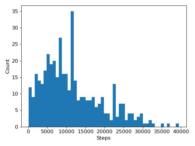
and the daily step count over time:
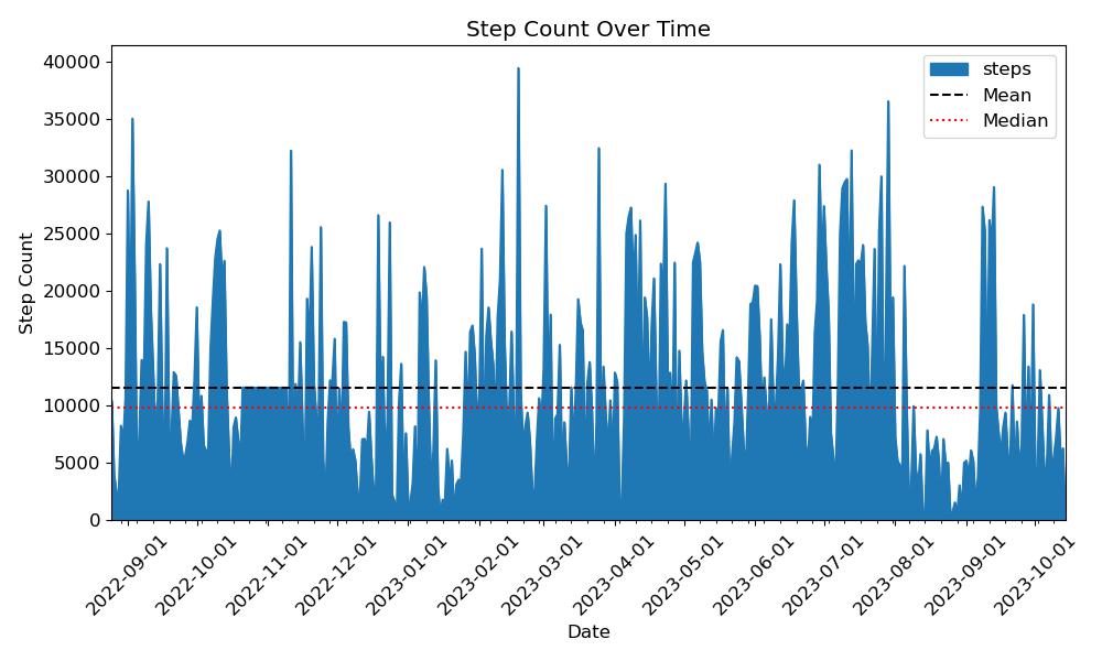
or the same information as a heatmap:
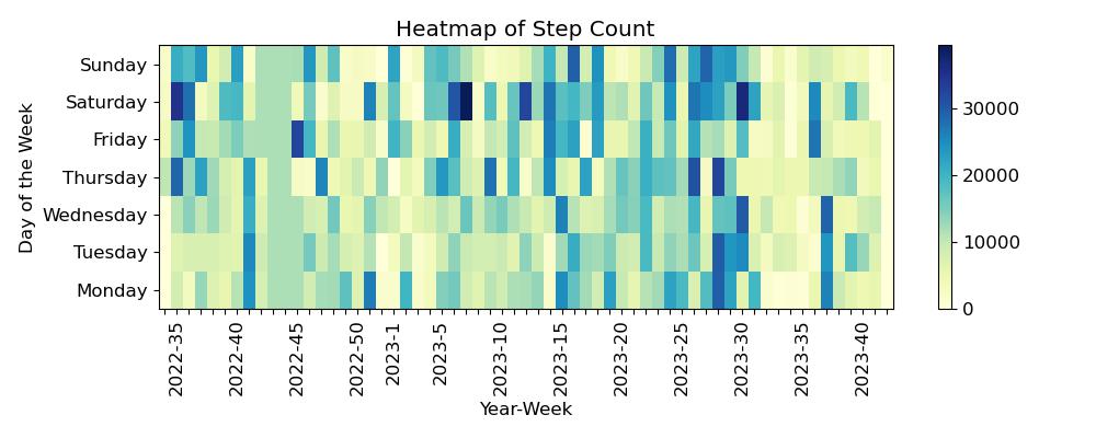
The day I took the most steps was the day of the Carnival of Cádiz. The night before we also were in a club so the night already contributed a lot:
      weekday
      weekend
      month
      season
      city
      country
      max_temp
      apparent_max_temp
      temp_difference
      humidity
      weather_condition
      simplified_weather
      steps
      activity
      money_spent_offline
      money_spent_online
      money_spent_total
      wifi_count_mean
      watch_1_steps
      watch_2_steps
      watch_steps_combined
      watch_1_mean_heart_rate
      watch_2_mean_heart_rate
      heart_rate_combined
      watch_type
      photos_videos
      media_activity
      generic_lat
      generic_lon


      date


      2023-02-18
      Saturday
      Weekend
      February
      Winter
      Cádiz
      Spain
      19.1
      15.1
      4.0
      Dry
      Light drizzle
      Rain
      39452
      High
      16.14
      0.0
      16.14
      13.15
      37912.0
      NaN
      37912.0
      78.0
      NaN
      78.0
      0.0
      24
      Moderate
      36.52672
      -6.2891
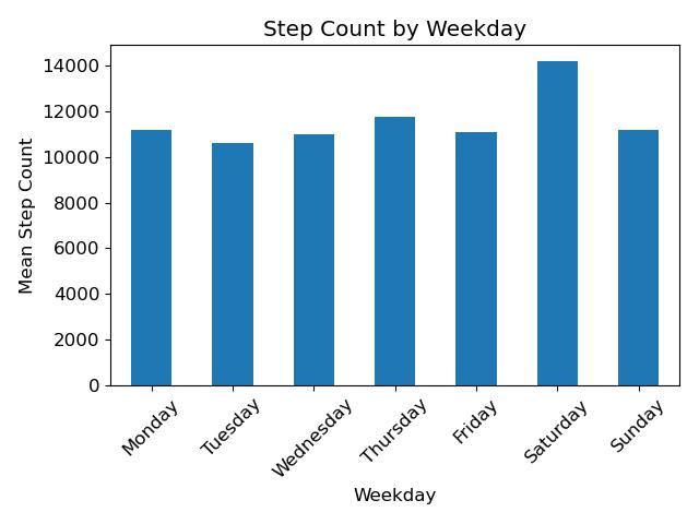
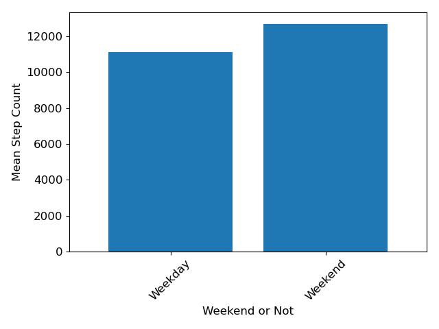
Next we can also observe if the step count differs between different days of the week. To me, it looks like there is a significant difference between Saturday and the rest of the week.
There would be a statistical test necessary to find out how likely this difference would be to appear due to randomness, but I will leave this out because I spent way too much time on this whole thing already.
This is the comparison between the weekend and not weekend:
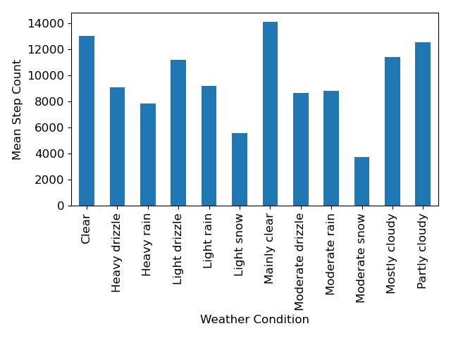
And the following is the comparison between different weather conditions. The following two graphs show the same information, but the second one contains simplified weather conditions which summarizes different strengths of the same weather condition (e.g. light rain and heavy rain are both rain).
As I would expect, the step count is higher when the weather is better.
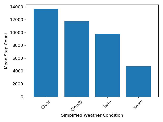
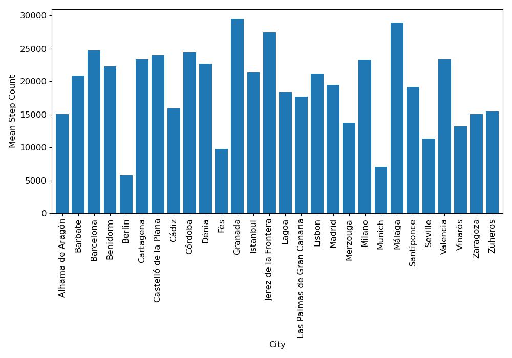
We can also compare the step count between different cities. The following graph shows the mean step count per city.
The most mean steps are in cities where I only stayed for a short time because I walked around a lot to see as much as possible in the short time I had.
Temperature
Changing to another variable, here is the daily maximum and apparent maximum temperature per day:
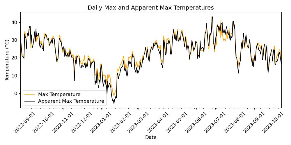
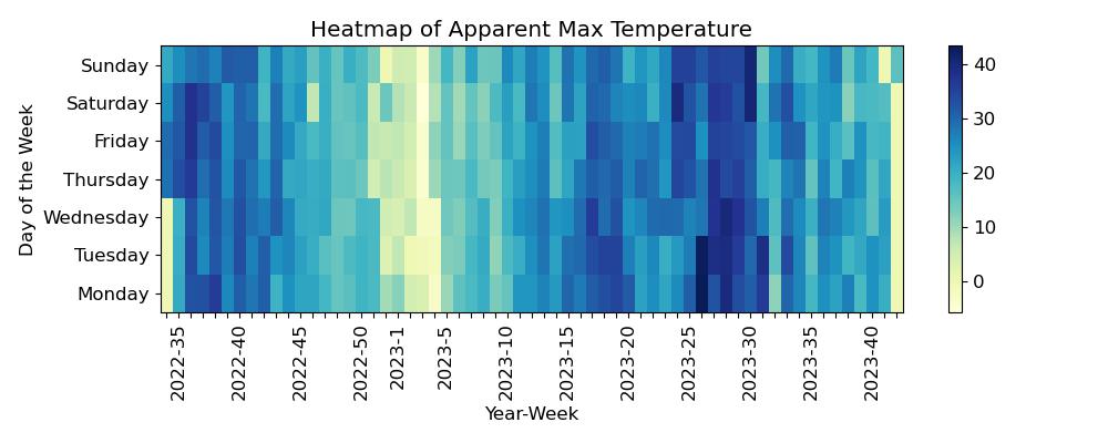
The hottest day I had was in Seville when the temperature rose to 43.3°C. I'm sure there were hotter days even, but I also escaped to Cádiz sometimes.
      weekday
      weekend
      month
      season
      city
      country
      max_temp
      apparent_max_temp
      temp_difference
      humidity
      weather_condition
      simplified_weather
      steps
      activity
      money_spent_offline
      money_spent_online
      money_spent_total
      wifi_count_mean
      watch_1_steps
      watch_2_steps
      watch_steps_combined
      watch_1_mean_heart_rate
      watch_2_mean_heart_rate
      heart_rate_combined
      watch_type
      photos_videos
      media_activity
      generic_lat
      generic_lon


      date


      2023-06-26
      Monday
      Weekday
      June
      Summer
      Seville
      Spain
      43.3
      43.3
      0.0
      Moderate
      Clear
      Clear
      7300
      Moderate
      187.41
      164.62
      352.03
      15.72
      NaN
      8419.0
      8419.0
      NaN
      67.0
      67.0
      1.0
      4
      Moderate
      37.38283
      -5.97317
I never experienced temperatures this high before. But, I was also surprised how it was less of a problem than expected. I think the reason for this is that the humidity was not that high.
This means the apparent temperature was similar to the actual temperature. We can plot the difference between the apparent and actual temperature. In this next graph, if the difference is positive, the apparent temperature is lower than the actual temperature.
From this I would conclude that the humidity is smaller. If the difference is negative I assume that the humidity is higher.
I'm not sure if this is completely correct under all circumstances (probably not, e.g., if there's a lot of wind), but I use it as an approximation for humidity.
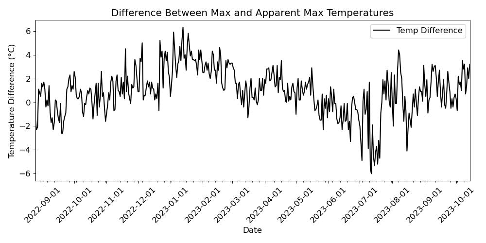
With this logic, the driest day was on January 13, 2023 in Munich with a difference of 6.3°C:
      weekday
      weekend
      month
      season
      city
      country
      max_temp
      apparent_max_temp
      temp_difference
      humidity
      weather_condition
      simplified_weather
      steps
      activity
      money_spent_offline
      money_spent_online
      money_spent_total
      wifi_count_mean
      watch_1_steps
      watch_2_steps
      watch_steps_combined
      watch_1_mean_heart_rate
      watch_2_mean_heart_rate
      heart_rate_combined
      watch_type
      photos_videos
      media_activity
      generic_lat
      generic_lon


      date


      2023-01-13
      Friday
      Weekday
      January
      Winter
      Munich
      Germany
      10.8
      4.5
      6.3
      Dry
      Moderate drizzle
      Rain
      13961
      High
      44.61
      98.07
      142.68
      15.38
      14159.0
      NaN
      14159.0
      70.0
      NaN
      70.0
      0.0
      0
      NaN
      48.13743
      11.57549
And the most humid day was on July 12, 2023 in Cartagena with a difference of -6.0°C. It was so humid there that you could feel the humidity in the air and on your skin. Sweating didn't have a cooling effect anymore. It also felt hotter than, for example, in Seville, although the actual temperature in Cartagena was way lower.
      weekday
      weekend
      month
      season
      city
      country
      max_temp
      apparent_max_temp
      temp_difference
      humidity
      weather_condition
      simplified_weather
      steps
      activity
      money_spent_offline
      money_spent_online
      money_spent_total
      wifi_count_mean
      watch_1_steps
      watch_2_steps
      watch_steps_combined
      watch_1_mean_heart_rate
      watch_2_mean_heart_rate
      heart_rate_combined
      watch_type
      photos_videos
      media_activity
      generic_lat
      generic_lon


      date


      2023-07-12
      Wednesday
      Weekday
      July
      Summer
      Cartagena
      Spain
      34.0
      40.0
      -6.0
      Humid
      Partly cloudy
      Cloudy
      16871
      High
      68.48
      8.0
      76.48
      10.63
      NaN
      17496.0
      17496.0
      NaN
      70.0
      70.0
      1.0
      16
      Moderate
      37.60512
      -0.98623
Weather
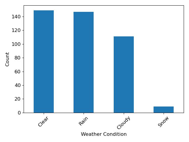
Next we can look at the (simplified) weather conditions I observed. The most common weather condition was clear, closely followed by rain. The few snowy days were probably mostly from the time I spent in Munich:
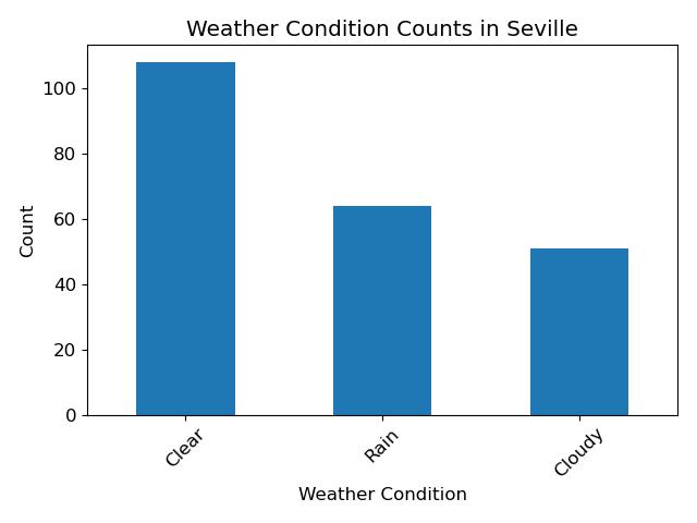
Looking only at the weather while I was in Seville, it was mostly clear, but there were also lots of rainy days. The longest period of consecutive days with rain was 7 days, starting on 2022-12-11.
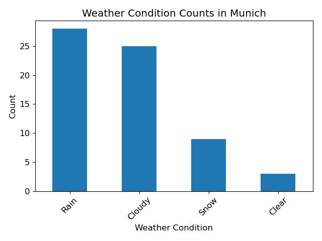
In Munich, it was mostly rainy/snowy, because I was there mostly in winter:
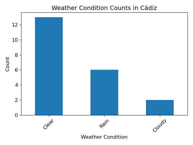
From the days I spent in Cádiz there were also quite a few rainy days:
Photos/Videos
Next we can look at the number of photos/videos taken per day. The following graph shows the number of photos/videos taken per day.
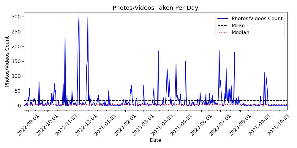

The day I took the most photos/videos was November 20, 2022 in Córdoba. I took 300 photos/videos that day.
      weekday
      weekend
      month
      season
      city
      country
      max_temp
      apparent_max_temp
      temp_difference
      humidity
      weather_condition
      simplified_weather
      steps
      activity
      money_spent_offline
      money_spent_online
      money_spent_total
      wifi_count_mean
      watch_1_steps
      watch_2_steps
      watch_steps_combined
      watch_1_mean_heart_rate
      watch_2_mean_heart_rate
      heart_rate_combined
      watch_type
      photos_videos
      media_activity
      generic_lat
      generic_lon


      date


      2022-11-20
      Sunday
      Weekend
      November
      Autumn
      Córdoba
      Spain
      16.4
      15.5
      0.9
      Moderate
      Mostly cloudy
      Cloudy
      23850
      High
      131.1
      4.99
      136.09
      11.8
      26638.0
      NaN
      26638.0
      80.0
      NaN
      80.0
      0.0
      300
      High
      37.89155
      -4.77275
I took at least one photo/video on 342 out of 416 days which is around 82.21% of all days.
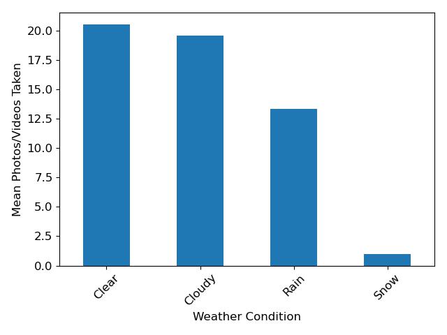
In total, I took 7198 photos/videos which is an average of 17.3 photos/videos per day, however the median is 4.
There is also an observable difference between different weather conditions again. The following graph shows the mean number of photos/videos taken per day for different (simplified) weather conditions.
I again won't do a statistical test.
Wi-Fi
Next up is the mean Wi-Fi count per day which is plotted in the following graph. The mean Wi-Fi count is the mean count of all the Wi-Fi networks my phone detected in the same day.
I imagined that this could be an indicator of how civilized my location is.
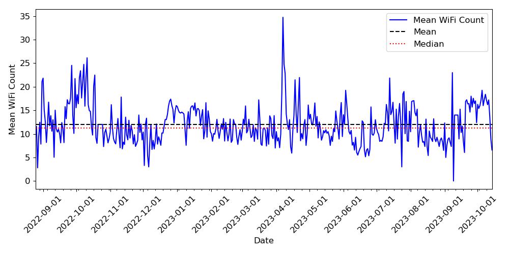
The day with the most Wi-Fi networks detected was April 7, 2023 in Barcelona with a mean of 34.75 Wi-Fi networks detected.
      weekday
      weekend
      month
      season
      city
      country
      max_temp
      apparent_max_temp
      temp_difference
      humidity
      weather_condition
      simplified_weather
      steps
      activity
      money_spent_offline
      money_spent_online
      money_spent_total
      wifi_count_mean
      watch_1_steps
      watch_2_steps
      watch_steps_combined
      watch_1_mean_heart_rate
      watch_2_mean_heart_rate
      heart_rate_combined
      watch_type
      photos_videos
      media_activity
      generic_lat
      generic_lon


      date


      2023-04-07
      Friday
      Weekday
      April
      Spring
      Barcelona
      Spain
      18.9
      17.0
      1.9
      Moderate
      Mainly clear
      Clear
      26486
      High
      34.06
      0.0
      34.06
      34.75
      26786.0
      NaN
      26786.0
      72.0
      NaN
      72.0
      0.0
      74
      High
      41.38879
      2.15899
Heart Rate
In October 2022 I also started measuring my heart rate. In May 2023 I switched to a different device.
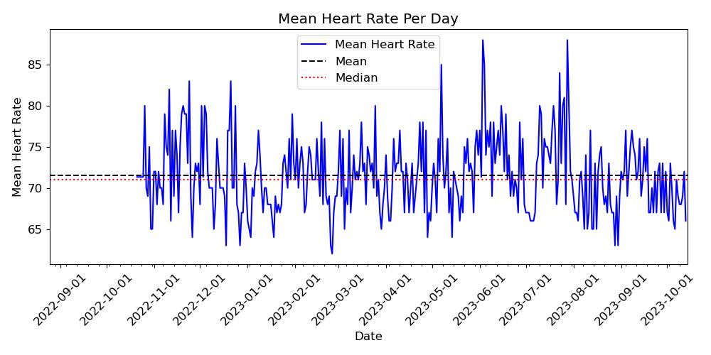
From the plot there is already a day that especially sticks out: June 3, 2023. On this day I had a mean heart rate of 88 bpm. It was the day I traveled from Seville to Munich to surprise my girlfriend on her birthday.
One could say that my heart rate could have been higher because I traveled on that day and because I was very active, but I also had lots of other days with these circumstances where my heart rate didn't stick out like this.
I think it's super cute to see that my heart rate was noticeably higher because I was so excited.
      weekday
      weekend
      month
      season
      city
      country
      max_temp
      apparent_max_temp
      temp_difference
      humidity
      weather_condition
      simplified_weather
      steps
      activity
      money_spent_offline
      money_spent_online
      money_spent_total
      wifi_count_mean
      watch_1_steps
      watch_2_steps
      watch_steps_combined
      watch_1_mean_heart_rate
      watch_2_mean_heart_rate
      heart_rate_combined
      watch_type
      photos_videos
      media_activity
      generic_lat
      generic_lon


      date


      2023-06-03
      Saturday
      Weekend
      June
      Summer
      Munich
      Germany
      21.0
      19.7
      1.3
      Moderate
      Mainly clear
      Clear
      16038
      High
      93.50
      0.0
      93.50
      19.25
      NaN
      13295.0
      13295.0
      NaN
      88.0
      88.0
      1.0
      4
      Moderate
      48.13743
      11.57549
The most relaxing day was on February 25, 2023 in Seville with a mean heart rate of 62 bpm.
I also happen to know what I did that day: I went to my favorite café, El Viajero Sedentario, for two and a half hours in the morning and afterward I relaxed on the rooftop enjoying the weather that was slowly getting warmer. Although there were a few rain drops on that day, there was also a long time of sun I could enjoy.
      weekday
      weekend
      month
      season
      city
      country
      max_temp
      apparent_max_temp
      temp_difference
      humidity
      weather_condition
      simplified_weather
      steps
      activity
      money_spent_offline
      money_spent_online
      money_spent_total
      wifi_count_mean
      watch_1_steps
      watch_2_steps
      watch_steps_combined
      watch_1_mean_heart_rate
      watch_2_mean_heart_rate
      heart_rate_combined
      watch_type
      photos_videos
      media_activity
      generic_lat
      generic_lon


      date


      2023-02-25
      Saturday
      Weekend
      February
      Winter
      Seville
      Spain
      15.2
      11.6
      3.6
      Dry
      Light drizzle
      Rain
      1975
      Low
      9.9
      0.0
      9.9
      7.77
      1887.0
      NaN
      1887.0
      62.0
      NaN
      62.0
      0.0
      1
      Moderate
      37.38283
      -5.97317
Money Spent
I tracked spending money "offline" and "online". Offline here means that I paid in person with my card and online means that I paid online with my card.
I tried only paying with card so most of my payments should be covered.
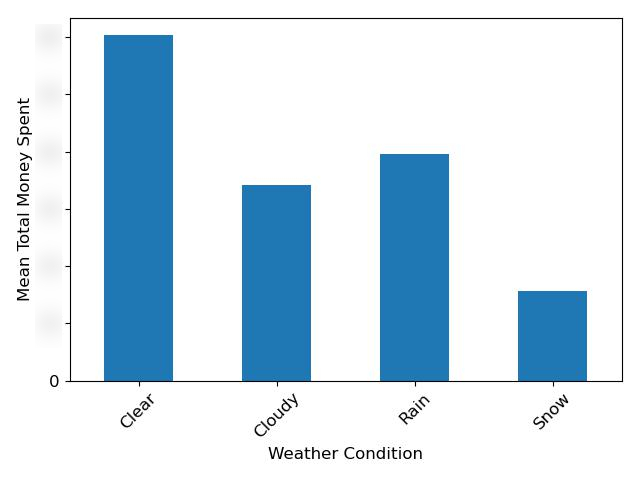
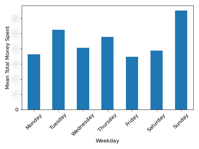
Comparing total money spent between different weather conditions we can see that the mean total money spent per day is the highest on clear days and on Sundays.
Y-scales are censored on purpose.
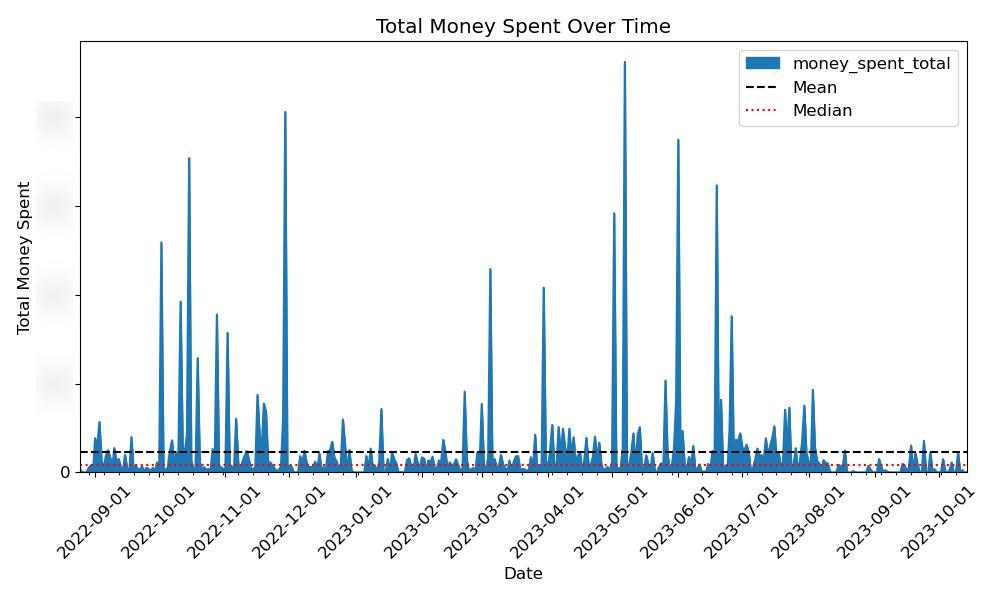
Y-scales are censored on purpose.
Y-scales are censored on purpose.

Offline Money Spent
For the offline spending the largest payment (excluding ATM withdrawals) was a flamenco show group evening at a bar that I prepaid for my friends.
      weekday
      weekend
      month
      season
      city
      country
      max_temp
      apparent_max_temp
      temp_difference
      humidity
      weather_condition
      simplified_weather
      steps
      activity
      money_spent_offline
      money_spent_online
      money_spent_total
      wifi_count_mean
      watch_1_steps
      watch_2_steps
      watch_steps_combined
      watch_1_mean_heart_rate
      watch_2_mean_heart_rate
      heart_rate_combined
      watch_type
      photos_videos
      media_activity
      generic_lat
      generic_lon


      date


      2023-05-26
      Friday
      Weekday
      May
      Spring
      Seville
      Spain
      28.1
      27.4
      0.7
      Moderate
      Moderate rain
      Rain
      10283
      Moderate
      ?????
      13.9
      ?????
      12.76
      NaN
      10209.0
      10209.0
      NaN
      73.0
      73.0
      1.0
      23
      Moderate
      37.38283
      -5.97317
Online Money Spent
The largest online payment was prepaying for our vacation rental in Cádiz.
      weekday
      weekend
      month
      season
      city
      country
      max_temp
      apparent_max_temp
      temp_difference
      humidity
      weather_condition
      simplified_weather
      steps
      activity
      money_spent_offline
      money_spent_online
      money_spent_total
      wifi_count_mean
      watch_1_steps
      watch_2_steps
      watch_steps_combined
      watch_1_mean_heart_rate
      watch_2_mean_heart_rate
      heart_rate_combined
      watch_type
      photos_videos
      media_activity
      generic_lat
      generic_lon


      date


      2023-05-07
      Sunday
      Weekend
      May
      Spring
      Seville
      Spain
      32.1
      31.0
      1.1
      Moderate
      Clear
      Clear
      24232
      High
      28.4
      ?????
      ?????
      11.63
      NaN
      21945.0
      21945.0
      NaN
      85.0
      85.0
      1.0
      150
      High
      37.38283
      -5.97317
At some point I also had to buy a new phone because I destroyed my old one while jumping around to music with my housemates. This was the second most expensive day.
      weekday
      weekend
      month
      season
      city
      country
      max_temp
      apparent_max_temp
      temp_difference
      humidity
      weather_condition
      simplified_weather
      steps
      activity
      money_spent_offline
      money_spent_online
      money_spent_total
      wifi_count_mean
      watch_1_steps
      watch_2_steps
      watch_steps_combined
      watch_1_mean_heart_rate
      watch_2_mean_heart_rate
      heart_rate_combined
      watch_type
      photos_videos
      media_activity
      generic_lat
      generic_lon


      date


      2022-10-15
      Saturday
      Weekend
      October
      Autumn
      Seville
      Spain
      28.9
      28.2
      0.7
      Moderate
      Clear
      Clear
      6076
      Moderate
      8.28
      ?????
      ?????
      11.42
      NaN
      NaN
      NaN
      NaN
      NaN
      NaN
      NaN
      0
      NaN
      37.38283
      -5.97317
And the day of the Barcelona vacation rental and flight payments comes after that.
      weekday
      weekend
      month
      season
      city
      country
      max_temp
      apparent_max_temp
      temp_difference
      humidity
      weather_condition
      simplified_weather
      steps
      activity
      money_spent_offline
      money_spent_online
      money_spent_total
      wifi_count_mean
      watch_1_steps
      watch_2_steps
      watch_steps_combined
      watch_1_mean_heart_rate
      watch_2_mean_heart_rate
      heart_rate_combined
      watch_type
      photos_videos
      media_activity
      generic_lat
      generic_lon


      date


      2023-03-05
      Sunday
      Weekend
      March
      Spring
      Seville
      Spain
      16.2
      14.6
      1.6
      Moderate
      Light rain
      Rain
      1972
      Low
      17.28
      ?????
      ?????
      10.22
      2076.0
      NaN
      2076.0
      65.0
      NaN
      65.0
      0.0
      2
      Moderate
      37.38283
      -5.97317
Correlations
Let's look at correlations between the different variables. The following correlations are the most interesting ones for me:
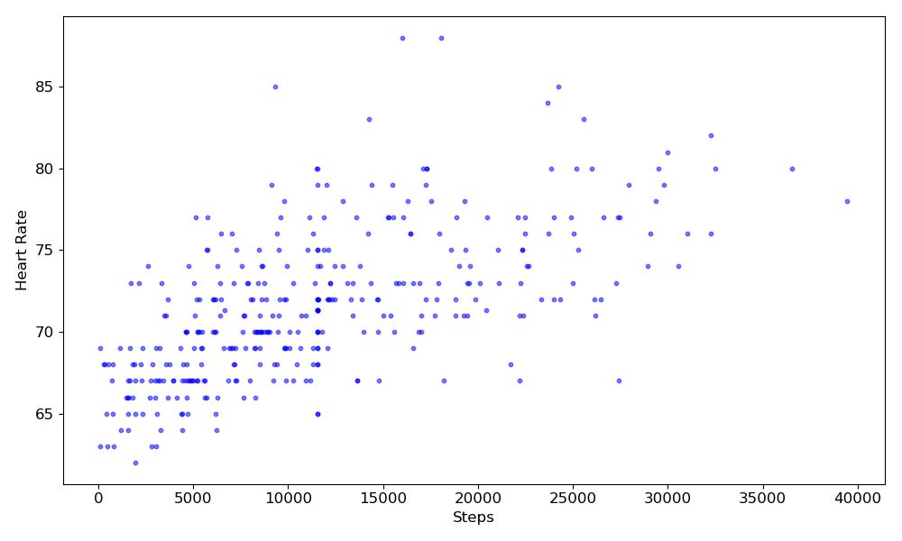
steps, heart_rate_combined: 0.62***
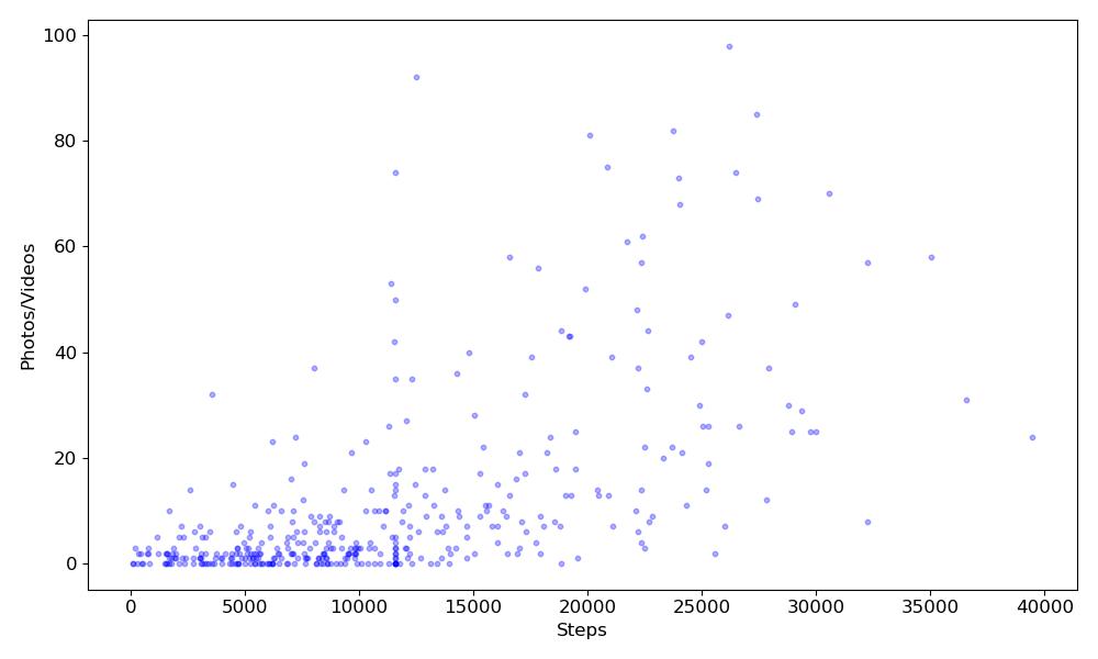
steps, photos_videos: 0.46***
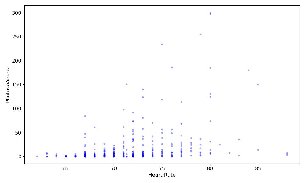
photos_videos, heart_rate_combined: 0.37***
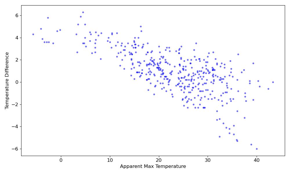
temp_difference, apparent_max_temp: -0.70***
Interpretation: Usually, on days I took more steps I also had a higher heart rate. This is very expected because I was more active on these days.
Also, on days I took more steps I also took more photos and videos. I like taking photos so this is also not surprising.
On days I took more photos I also usually had a higher heart rate, but this correlation is rather weak.
Finally, on days with a higher difference between the max and apparent max temperature there was usually a lower apparent max temperature. I think a reason for this can be that I was mostly in dry-ish climates.
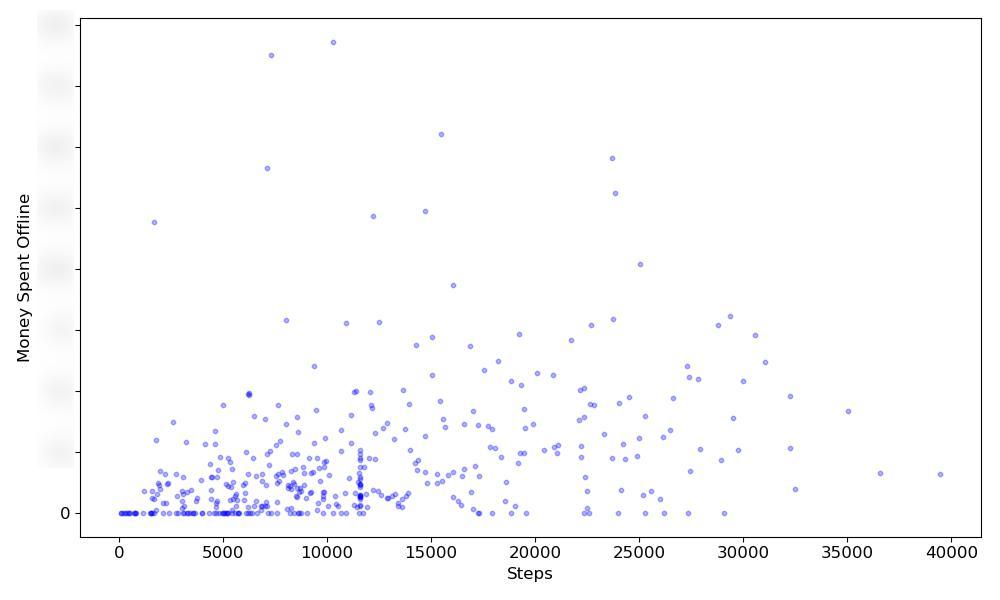
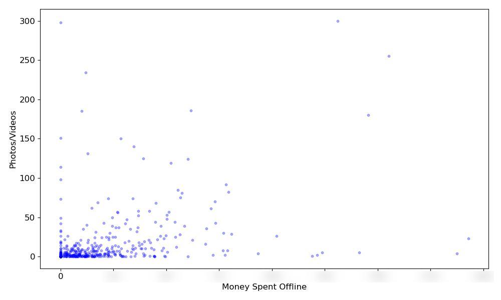
Unlike in the previous data post, there are no significant correlations with money_spent anymore.
That may be a less interesting result now, but it's good because it increases the potential for more accurately predicting my location later.
Here are two example plots showing the weak correlation with money spent (money scales are censored on purpose):
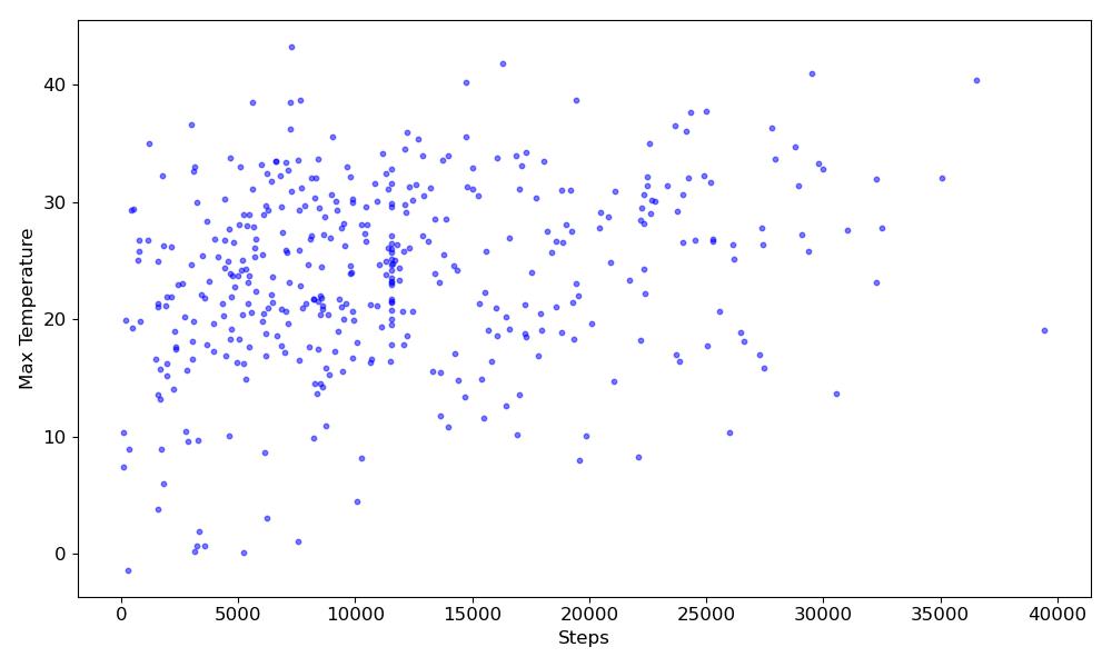
One could also expect a correlation between the max temperature and the number of steps. However, this correlation is very weak (0.25):
Linear Regression
My goal with linear regression here is not to make accurate predictions, but to find interesting relationships between the variables.
Of course, these relationships are not causal.
Also, I didn't test the assumptions of linear regression here, so the results are not very reliable.
Steps as independent variable
First I run a linear regression with the number of steps as the dependent variable. Through backwards elimination of independent variables that are insignificant at the 1% level I end up with the following model.
apparent_max_temp, wifi_count_mean, and photos_videos are the only significant independent variables.
An interpretation of the result would be that if the apparent max temperature increased by 1°C, I took on average 209.36 more steps, holding the other variables constant.
If the mean Wi-Fi count increased by 1, I took on average 362.81 more steps, holding the other variables constant.
If the number of photos and videos I took increased by 1, I took on average 89.26 more steps, holding the other variables constant.
                            OLS Regression Results
==============================================================================
Dep. Variable:                  steps   R-squared:                       0.299
Model:                            OLS   Adj. R-squared:                  0.294
Method:                 Least Squares   F-statistic:                     58.49
Date:                Sun, 24 Dec 2023   Prob (F-statistic):           1.61e-31
Time:                        13:37:10   Log-Likelihood:                -4243.7
No. Observations:                 416   AIC:                             8495.
Df Residuals:                     412   BIC:                             8512.
Df Model:                           3
Covariance Type:            nonrobust
=====================================================================================
                        coef    std err          t      P>|t|      [0.025      0.975]
-------------------------------------------------------------------------------------
const               877.9449   1305.529      0.672      0.502   -1688.385    3444.274
apparent_max_temp   209.3622     35.732      5.859      0.000     139.123     279.601
wifi_count_mean     362.8066     76.920      4.717      0.000     211.603     514.011
photos_videos        89.2580      8.573     10.412      0.000      72.406     106.110
==============================================================================
Omnibus:                       40.938   Durbin-Watson:                   1.468
Prob(Omnibus):                  0.000   Jarque-Bera (JB):               54.677
Skew:                           0.725   Prob(JB):                     1.34e-12
Kurtosis:                       4.027   Cond. No.                         177.
==============================================================================

Notes:
[1] Standard Errors assume that the covariance matrix of the errors is correctly specified.
Photos/Videos ~ steps
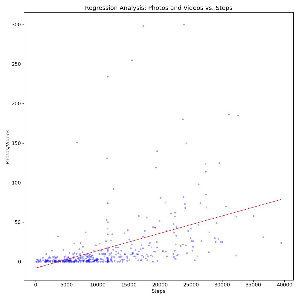
Next, I run a linear regression with the number of photos and videos as the dependent variable and just the steps as the independent variable.
As noted in note [2], there seem to be some problems with the model. Like I said before, I didn't test the assumptions of linear regression here, so the results are not very reliable.
Nevertheless, the model estimates that if my number of steps increased by 1, the number of photos and videos I took increased by 0.0022 on average.
The negative intercept is significant, but has no practical meaning in this case.
                            OLS Regression Results
==============================================================================
Dep. Variable:          photos_videos   R-squared:                       0.208
Model:                            OLS   Adj. R-squared:                  0.206
Method:                 Least Squares   F-statistic:                     108.4
Date:                Sun, 24 Dec 2023   Prob (F-statistic):           1.05e-22
Time:                        13:37:11   Log-Likelihood:                -2050.7
No. Observations:                 416   AIC:                             4105.
Df Residuals:                     414   BIC:                             4114.
Df Model:                           1
Covariance Type:            nonrobust
==============================================================================
                 coef    std err          t      P>|t|      [0.025      0.975]
------------------------------------------------------------------------------
const         -8.1747      2.949     -2.772      0.006     -13.971      -2.379
steps          0.0022      0.000     10.412      0.000       0.002       0.003
==============================================================================
Omnibus:                      428.657   Durbin-Watson:                   1.399
Prob(Omnibus):                  0.000   Jarque-Bera (JB):            15285.273
Skew:                           4.624   Prob(JB):                         0.00
Kurtosis:                      31.219   Cond. No.                     2.50e+04
==============================================================================

Notes:
[1] Standard Errors assume that the covariance matrix of the errors is correctly specified.
[2] The condition number is large, 2.5e+04. This might indicate that there are
strong multicollinearity or other numerical problems.
Heart Rate ~ steps
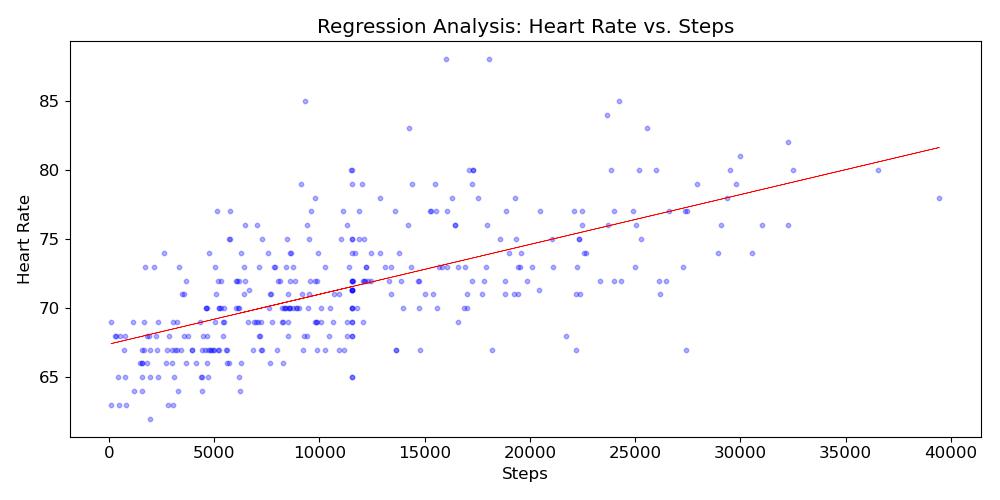
Let's look at the relationship between the heart rate and just the number of steps.
The model estimates that if my number of steps increased by 1, my mean heart rate for that day increased by 0.0004 bpm on average.
                             OLS Regression Results
===============================================================================
Dep. Variable:     heart_rate_combined   R-squared:                       0.387
Model:                             OLS   Adj. R-squared:                  0.385
Method:                  Least Squares   F-statistic:                     224.3
Date:                 Sun, 24 Dec 2023   Prob (F-statistic):           1.14e-39
Time:                         13:38:03   Log-Likelihood:                -960.01
No. Observations:                  358   AIC:                             1924.
Df Residuals:                      356   BIC:                             1932.
Df Model:                            1
Covariance Type:             nonrobust
==============================================================================
                 coef    std err          t      P>|t|      [0.025      0.975]
------------------------------------------------------------------------------
const         67.3933      0.334    201.593      0.000      66.736      68.051
steps          0.0004   2.41e-05     14.977      0.000       0.000       0.000
==============================================================================
Omnibus:                       49.215   Durbin-Watson:                   1.443
Prob(Omnibus):                  0.000   Jarque-Bera (JB):               81.853
Skew:                           0.822   Prob(JB):                     1.68e-18
Kurtosis:                       4.669   Cond. No.                     2.48e+04
==============================================================================

Notes:
[1] Standard Errors assume that the covariance matrix of the errors is correctly specified.
[2] The condition number is large, 2.48e+04. This might indicate that there are
strong multicollinearity or other numerical problems.
heart rate ~ watch_type + steps
As I switched to a different watch in May 2023, I also wanted to see if the devices differ in their heart rate measurements.
I wasn't sure if I should include this section, because the included independent variables are very limited and I only tried linear relationships. Resulting R-squared values are rather low. Although these limitations might lead to very unreliable results, I'll still include this section to show my thinking.
Another way to ask if the devices differ in their measurement is if the watch type influences the measured mean heart rate.
For this I run a linear regression with the mean heart rate as the dependent variable and the watch type and the number of steps as the independent variables because I want to account for the influence of the number of steps.
The estimated model's watch_type coefficient is not significant, so the watch type doesn't seem to influence the measured mean heart rate (which would be good because if both are accurate there shouldn't be a difference).
                             OLS Regression Results
===============================================================================
Dep. Variable:     heart_rate_combined   R-squared:                       0.388
Model:                             OLS   Adj. R-squared:                  0.384
Method:                  Least Squares   F-statistic:                     112.3
Date:                 Sun, 24 Dec 2023   Prob (F-statistic):           1.61e-38
Time:                         13:38:25   Log-Likelihood:                -959.71
No. Observations:                  358   AIC:                             1925.
Df Residuals:                      355   BIC:                             1937.
Df Model:                            2
Covariance Type:             nonrobust
==============================================================================
                 coef    std err          t      P>|t|      [0.025      0.975]
------------------------------------------------------------------------------
const         67.2716      0.370    181.645      0.000      66.543      68.000
watch_type     0.2888      0.377      0.765      0.445      -0.453       1.031
steps          0.0004   2.41e-05     14.937      0.000       0.000       0.000
==============================================================================
Omnibus:                       47.203   Durbin-Watson:                   1.441
Prob(Omnibus):                  0.000   Jarque-Bera (JB):               77.079
Skew:                           0.800   Prob(JB):                     1.83e-17
Kurtosis:                       4.614   Cond. No.                     3.31e+04
==============================================================================

Notes:
[1] Standard Errors assume that the covariance matrix of the errors is correctly specified.
[2] The condition number is large, 3.31e+04. This might indicate that there are
strong multicollinearity or other numerical problems.
heart rate ~ watch_type + photos_videos + apparent_max_temp
I also tried to use the number of photos/videos I took and the apparent max temperature as a proxy for how active I was on a day.
Here the watch type coefficient isn't significant either.
                             OLS Regression Results
===============================================================================
Dep. Variable:     heart_rate_combined   R-squared:                       0.161
Model:                             OLS   Adj. R-squared:                  0.154
Method:                  Least Squares   F-statistic:                     22.59
Date:                 Sun, 24 Dec 2023   Prob (F-statistic):           2.10e-13
Time:                         13:38:28   Log-Likelihood:                -1016.1
No. Observations:                  358   AIC:                             2040.
Df Residuals:                      354   BIC:                             2056.
Df Model:                            3
Covariance Type:             nonrobust
=====================================================================================
                        coef    std err          t      P>|t|      [0.025      0.975]
-------------------------------------------------------------------------------------
const                69.1102      0.579    119.364      0.000      67.972      70.249
watch_type           -0.0576      0.515     -0.112      0.911      -1.071       0.956
photos_videos         0.0408      0.006      7.338      0.000       0.030       0.052
apparent_max_temp     0.0784      0.028      2.803      0.005       0.023       0.133
==============================================================================
Omnibus:                       33.655   Durbin-Watson:                   1.559
Prob(Omnibus):                  0.000   Jarque-Bera (JB):               43.765
Skew:                           0.699   Prob(JB):                     3.14e-10
Kurtosis:                       3.990   Cond. No.                         122.
==============================================================================

Notes:
[1] Standard Errors assume that the covariance matrix of the errors is correctly specified.
Goal 2: Prediction
Now let's get to the second part: predicting my location on a city level based on my behavior.
I filtered out all days I stayed in a city that I stayed in for less than 7 days. This leaves 5 possible cities to predict: Seville, Munich, Berlin, Cádiz, and Istanbul.
Then I applied encoding and standardization where necessary/applicable.
My goal here isn't to produce the absolute best model, but rather to try out different approaches and see what might work better than other approaches here.
Neural Network
The first approach I tried was to use a neural network. For this I also used SMOTE to balance the classes.
NN: First Try
Just for the first neural network try I used all variables except variables coming from the watch, or variables directly hinting at my location (coordinates and country).
Without much trying around I ended up with the following architecture:
Three dense layers, two of which with a ReLU activation, and the last one with a softmax activation.
Model: "sequential"
_________________________________________________________________
 Layer (type)                Output Shape              Param #
=================================================================
 dense (Dense)               (None, 64)                3776

 dense_1 (Dense)             (None, 32)                2080

 dense_2 (Dense)             (None, 5)                 165

=================================================================
Total params: 6,021
I used the Adam optimizer, a categorical cross entropy loss, and accuracy metrics. After training for 10 epochs I got the following results:
Orange: train accuracy
Blue: validation accuracy
Orange: train loss
Blue: validation loss
NN Second Try: Only Behavioral Variables
For the second try with a neural network I only left the behavioral variables (steps, money spent, photos/videos).
This was my goal from the beginning.
I also tried out a different architecture with one ReLU layer, one softmax layer, and L2 regularization.
Model: "sequential_3"
_________________________________________________________________
 Layer (type)                Output Shape              Param #
=================================================================
 dense_7 (Dense)             (None, 64)                704

 dense_8 (Dense)             (None, 5)                 325

=================================================================
Total params: 1,029
Trainable params: 1,029
Non-trainable params: 0
_________________________________________________________________
Orange: train accuracy
Blue: validation accuracy
Orange: train loss
Blue: validation loss
Here we end up with a pretty bad validation accuracy. It also looks a lot like the model is overfitting.
I didn't try to improve this a lot because of time reasons and because I think the most promising way to fix this would be to have more data which I can't do anyway unless I wait for multiple years.
New example not included in dataset
Nevertheless, the model can already correctly predict the city of my test day:
December 19, 2023
example = {
    'steps': 2575,
    'money_spent_offline': 0,
    'money_spent_online': 0,
    'money_spent_total': 0,
    'photos_videos': 0
}
Actual: Munich
Predicted: Munich
However, with a validation accuracy this low, this might as well be just a random guess.
KNN
The next method I tried was KNN, where the highest accuracy I got was 0.42 with K=3.
This is already better than the NN, but I suspected the next methods would lead to better results.
Random Forest
For random forest I did a random search for the best parameters.
Here I ended up with an accuracy of 0.65.
XGBoost
And for XGBoost I got an accuracy of 0.69 (nice).
With a random search I even found parameters that lead to an accuracy of 0.7. This appears to be the best model I could find without investing more time into this.
And I think it's already pretty good. It can also correctly predict the city of my test day:
New example not included in dataset
December 19, 2023
example = {
    'steps': 2575,
    'money_spent_offline': 0,
    'money_spent_online': 0,
    'money_spent_total': 0,
    'photos_videos': 0
}
Actual: Munich
Predicted: Munich
But of course, it's not always correct:
December 05, 2023
example = {
    'steps': 3579,
    'money_spent_offline': 14.1,
    'money_spent_online': 0,
    'money_spent_total': 14.1,
    'photos_videos': 0
}
Actual: Munich
Predicted: Berlin
For this day it got the city wrong, but at least it was still in the same country.
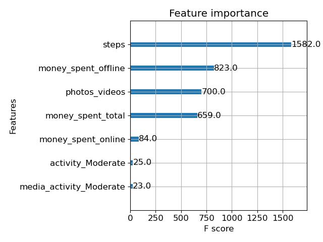
Counting how often a feature is used to split the data across all trees, we can see that the number of steps is the most important feature, followed by money spent offline, the number of photos/videos taken, and money spent online. 'activity' and 'media_activity' are just augmentations I derived from the number of steps and photos/videos.
Conclusion
The XGBoost model turned out to work best for this work. As I didn't try improving much on the neural network, further exploring might lead to better results. Also, the accuracy metric I used could be complemented by other metrics.
I could have incorporated more behavioral features like which transportation modes I used on the day, but I didn't want to spend too much time on this project.
For now, I'm very content with the result already.
It shows that my behavior changes enough between different cities to be able to predict the city I'm in. It is not applicable to anyone besides myself, but I suspect that lots of people would have similar results if they were to try this.
Although doing this was fun, I'm not sure if there are any practical applications for the prediction of my location, as every device has GPS built in and knows its location.
As GPS usage is rather battery-consuming, there might be use cases for predicting the location without GPS usage. As this is done on a city-level, it might be useful for, e.g., weather services.
At least this post might inspire similar fun personal projects for others which can help to learn about data collection, exploration, and prediction.
I wouldn't continue trying to improve this model, but I can imagine to keep collecting my data for further explorations and visualizations over the years.
I hope you enjoyed this little project.
What is left to write for me is a general summary post of the whole time.